
Coding agents can help investigate large amounts of observability data, from finding recurring failures to explaining an increase in cost. To do that well, they need to find relevant traces, compare them, and inspect individual calls.
The challenge is that an investigation rarely follows a fixed set of queries. A cost breakdown might point to one model, but understanding the increase may require looking at failed tool calls and the retries inside individual traces. What the agent needs to retrieve depends on what it finds.
We chose SQL to give coding agents that flexibility in Laminar. They can filter, aggregate, and combine related data through one interface, without us having to build and maintain an endpoint for every new question.
Too many endpoints
The usual way to expose application data is through GET endpoints. A client calls one endpoint to list traces and another to fetch a span. This works well when we know which queries the client needs.
Supporting a new question often means adding a filter, a grouping option, or another endpoint. As users investigate different models, tools, and failure patterns, those combinations multiply. Adding endpoints for each query pattern does not scale: we end up maintaining a growing API while still leaving some questions unsupported.
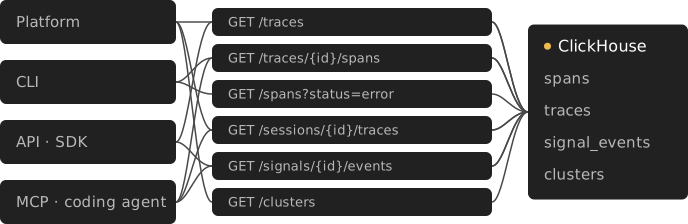
Exposing those endpoints as tools also has a cost for coding agents. Tool descriptions and parameter schemas take up context. When the tools cannot express a query, the agent has to fetch records and calculate the answer itself. Extra calls add latency, and processing larger responses consumes more tokens.
SQL as the interface
Coding agents already know how to write SQL. We give them the tables and columns available in Laminar, along with a little guidance on how to query our data.
For example, an agent investigating rising spend can query daily cost by model. The spans table contains the individual calls and operations within each trace:
SELECT toDate(start_time) AS day, model, sum(total_cost) AS cost
FROM spans
WHERE start_time > now() - INTERVAL 7 DAY
GROUP BY day, model
ORDER BY day, cost DESC
ClickHouse performs the aggregation before returning the results. From there, the agent can inspect the individual calls for a particular model and day.
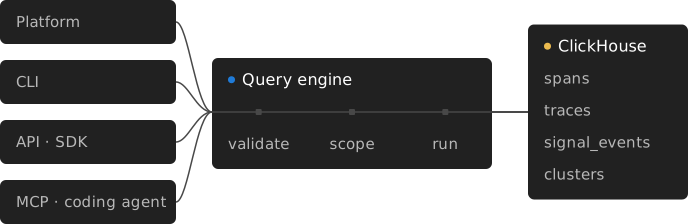
The same query engine powers data retrieval throughout Laminar, including our SQL editor, dashboards, CLI, and MCP server. As we add features, we can reuse that interface instead of building separate query logic and endpoints for each new access pattern.
How the query engine works
Our query engine runs inside Laminar’s Rust backend. It validates incoming SQL and maps table references to views before sending the query to ClickHouse.
Validating queries
We use sqlparser to parse SQL into a syntax tree and check it, including its subqueries. We enforce three restrictions:
- Read-only: only a single SELECT statement is accepted.
- Allowed tables: table references must belong to the set we expose.
- Restricted operations: file reads and external access are blocked; query settings are stripped.
Querying through views
ClickHouse’s parameterized views sit between our database tables and the users querying them. Each view is a saved SELECT query that lets us shape the data we expose. For example, the spans view turns internal enum values into readable names: 0 → 'DEFAULT', 1 → 'LLM', and 6 → 'TOOL'.
Views also let us filter data to the user’s project. When an agent queries spans, we route it through spans_v1 and pass in project_id from the request, so the view reads only that project’s data.
-- View definition
CREATE VIEW spans_v1 SQL SECURITY INVOKER AS
SELECT
    multiIf(
        span_kind = 0, 'DEFAULT',
        span_kind = 1, 'LLM',
        span_kind = 6, 'TOOL',
        'UNKNOWN'
    ) AS span_type,
    total_cost
FROM spans
WHERE project_id = {project_id:UUID};

-- Example query under the hood
SELECT span_type, sum(total_cost) AS cost
FROM spans_v1(project_id = '00000000-0000-0000-0000-000000000001')
GROUP BY span_type;
The query engine uses a separate ClickHouse user for these reads. Giving that user read-only permissions adds another layer of protection: ClickHouse can reject writes even if they get past query validation.
Denormalizing trace data
Signals are one of Laminar's core features for debugging agents. They analyze runs and emit events when they detect something you want to track, such as a tool failure. Clustering groups similar events into clusters, making recurring problems like tool timeouts easier to find.
These clusters give coding agents a starting point for investigating recurring failures. But comparing the cost of those failures requires data from three places: traces (agent runs), signal events, and clusters.
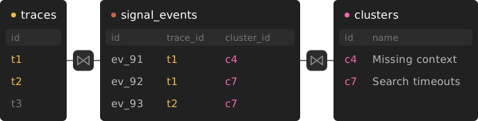
To answer “Which groups of traces are costing us the most?”, we had to join clusters to their events, then match those events to traces to retrieve the costs. A trace can have several events and belong to several clusters, so this involves more than a simple lookup. Each investigation has to assemble those relationships at query time.
Why not joins?
Both the trace and event tables grow with the number of traces, so each investigation could involve joining two large tables.
The signal_events table is indexed to support signal processing and clustering, both of which operate on the events of a particular signal. Looking up events by trace_id does not follow that access pattern, so those queries have to scan more data.
We considered some ways to keep the data separate:
- Spend more compute on joins. Each investigation would still pay the CPU and memory cost of joining the growing tables, and queries would remain too slow for interactive exploration.
- Fetch the data in separate queries. We could fetch matching events, then their traces. But this moves joining logic into clients, forcing us to anticipate join patterns. That’s the problem we built the query engine to avoid. Queries matching many events also require transferring large ID lists across multiple requests.
- Use a dictionary for lookups. Caching helps when queries reuse the same data. New trace IDs miss the cache, and cached results need refreshing to include new events. Those reads still have to assemble the data from the source tables.
Copying data onto traces
We instead copied the frequently queried event data and cluster membership onto the trace. Each stored trace now carries two arrays:
- signal_events: tuples containing the event_id, signal_id, severity, and payload.
- cluster_ids: the IDs of the most specific named clusters associated with the trace's events.

This adds writes, but our AggregatingMergeTree table lets us insert just the new events or cluster IDs. ClickHouse aggregates our partial records, so we can write updates without the overhead of reading the trace back.
In production, this increased storage for our trace table by about 3%. We considered that a reasonable tradeoff for reducing the CPU and memory spent on large joins during investigations.
A dictionary for clusters
The trace stores cluster_ids, but queries also need their names and hierarchy. These details are a good fit for a dictionary: clustering groups many similar events into relatively few clusters, so the lookup stays small even as more events arrive.
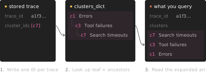
We use clusters_dict, an in-memory dictionary keyed by project_id and cluster_id. It follows parent_id to build each cluster's chain of parents, such as “Search timeouts” → “Tool failures” → “Errors.” Queries can look up this chain in memory instead of rebuilding it each time.
ClickHouse checks the cluster table every 30–60 seconds and reloads the dictionary only when the data changes. If “Search timeouts” is renamed, queries pick up the new name after the next refresh. That short delay is acceptable for exploring recurring patterns, where cluster details do not need to reflect every edit immediately.
We can now answer the cost question directly by ranking clusters over the past week:
SELECT
    c.name AS cluster,
    count() AS trace_count,
    sum(total_cost) AS cost,
    avg(total_cost) AS avg_trace_cost
FROM traces
ARRAY JOIN clusters AS c
WHERE start_time > now() - INTERVAL 7 DAY
    AND c.level = 1
GROUP BY c.id, c.name
ORDER BY cost DESC
LIMIT 10
The trace count and average cost help distinguish a frequent failure from one that affects a few expensive runs.
Bringing Postgres into the same query
Once an agent finds a recurring problem, it may want to read the signal's instructions to understand what was detected. Those definitions live in Postgres, whose transactions are a better fit for frequently edited data.
Even a question like “Which signals are firing most often?” required data from both databases. The agent could count events in ClickHouse, but it then had to fetch the signal names through a separate API call and match them by signal_id. We wanted that lookup to be part of the SQL query.
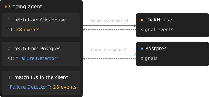
Reading Postgres through ClickHouse
Those reads also had to reflect recent edits. Agents often verify an update by reading the definition back, and a stale version could make a successful edit look like it failed.
We considered three approaches:
- Use a dictionary. This would reuse our approach for cluster details, but edits would only appear after a refresh.
- Copy definitions into ClickHouse. Queries could read the data locally, but we'd need to keep that copy in sync with every edit in Postgres.
- Combine results in our query engine. We'd have to build the logic to plan reads across both databases and join the results ourselves.
We chose ClickHouse's PostgreSQL database engine, which reads tables directly from Postgres when a query runs. ClickHouse can then join those definitions with its local event data.
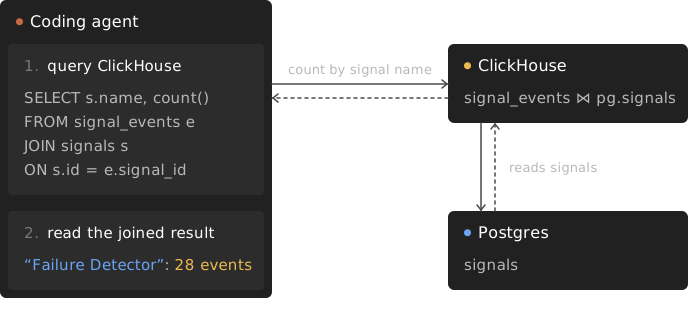
We expose signals, evaluations, and datasets through views that restrict results to the caller's project. To find the most frequently triggered signals, the agent can now write:
SELECT s.name, count() AS events
FROM signal_events e
JOIN signals s ON s.id = e.signal_id
GROUP BY s.name
ORDER BY events DESC
┌─s.name───────────┬─events─┐
│ test             │   2500 │
│ Failure Detector │     28 │
└──────────────────┴────────┘
The table descriptions we provide through MCP also tell the agent about the prompt column. It can then read the instructions behind “Failure Detector” to understand what those 28 events represent.
The cost of reading Postgres
Every query that uses these tables makes a request to Postgres. In our measurements, fetching 1,000 metadata rows took 3 to 4 ms, and 100,000 took about 30 ms.
The query's answer can be much smaller than the data it reads. With our views, Postgres sends rows from the caller's project and only the columns the query needs. ClickHouse does the rest of the work after those rows arrive. Filtering for one signal by name can therefore still fetch every signal definition in the project.
Our definition tables are small enough that we can afford to read them on each query and return up-to-date names and settings. As the number of definitions in a project grows, fetching those rows on every query becomes more expensive.
Putting it together
We can’t anticipate every question an agent will ask during an investigation. With SQL, we don’t have to build an endpoint for each one. We can focus on making the underlying data useful and efficient to query, while agents decide how to explore it. As new questions come up, the same interface gives them a way to keep going.